Getting Started with Python
Contents
1. Getting Started with Python#
1.1. Lesson overview#
Python is an excellent programming language to help accelerate your scientific research and projects. It is well suited for many tasks in the scientific domain, such as controlling instruments, analyzing large amounts of data, and automating routine tasks. Python is a free and open source language with minimalist syntax that makes it easy to get coding quickly, and has a thriving ecosystem of over 100,000 libraries including standard scientific libraries like Numpy and SciPy. We will explore some software tools that are needed to start working with Python. In this lesson, we will install Anaconda, which is a common Python distribution, and walk through running a Python interactive shell, creating and running code files with Spyder, and starting up some JupyterLab notebooks.
1.2. Installing Anaconda#
Anaconda is a bundled Python distribution that is available for all operating systems and comes installed with many common Python libraries. In this guide, we will be using the latest version of Anaconda. Below are instructions for installing Anaconda on Windows or Mac:
1.3. Launching Anaconda Navigator#
The next step after installing Anaconda is to start up Anaconda Navigator. Details on starting Anaconda Navigator for Windows and Mac operating systems are provided below:
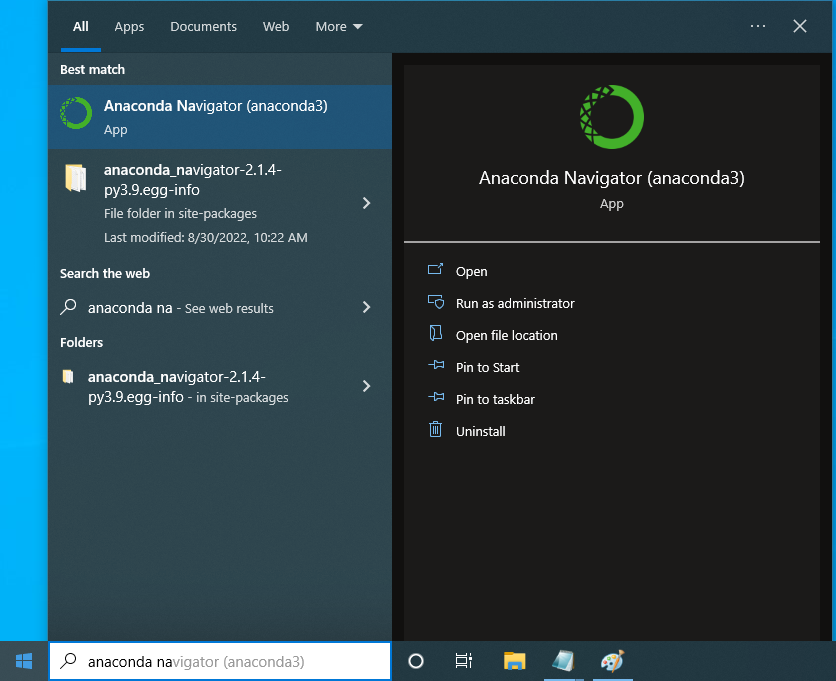
1.3.1. Windows#
In Windows, go to the “Start Menu” and type “Anaconda Navigator”
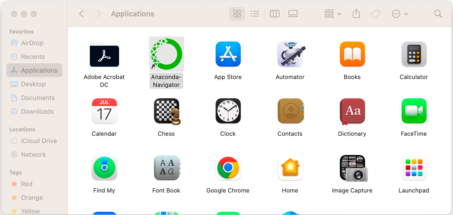
1.3.2. Mac#
In Mac, open “Finder”, then select “Applications”, and click on “Anaconda-Navigator”
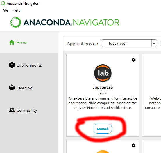
1.3.3. Anaconda Navigator#
Anaconda Navigator is the application platform for Anaconda. The default view after launching Anaconda is the Home view. The Environments, Learning, and Community views can also be accessed using the left-hand side links.
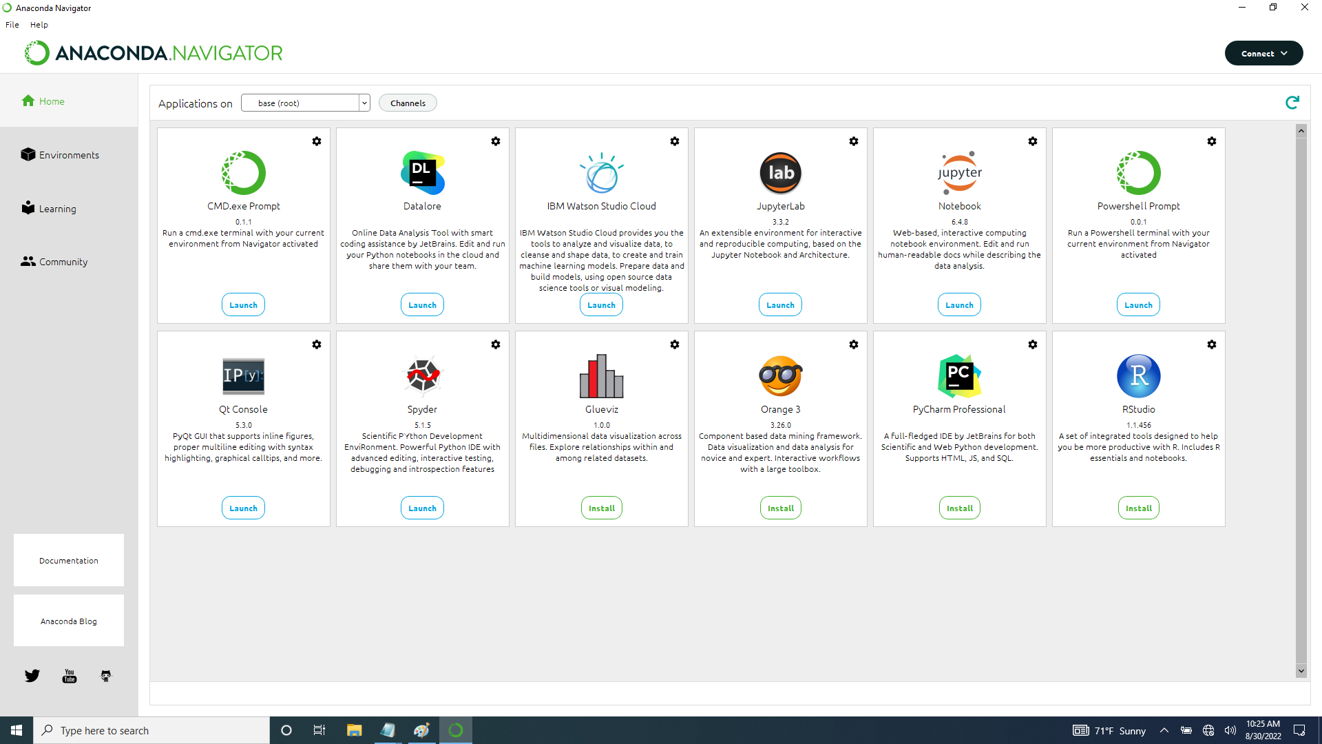
The Home view will be used the most as it displays the various launchers to different Python programs and development environments. Later, we will use three of these launchers: CMD.exe Prompt (for Windows), Spyder, and JupyterLab, to explore Python.
The Environments view displays the different Python virtual environments currently available and what Python libraries are installed in those environments. The default virtual environment is the “base (root)” environment, which we will be using.
Finally, the Learning and Community views display many hyperlinks to documentation and online Python forums that can be useful places to learn more about Python and different Python libraries.
Hey! Listen!
Virtual environments are useful to control which version of a Python library you have installed for a project. Each environment contains its own separate list of libraries, so dependency conflicts between libraries are avoided. It is recommended to create a virtual environment for each of your Python projects. You can check out the official Anaconda tutorial on how to manage virtual environments.
1.4. Running the Python interactive shell#
We can jump into the Python shell (i.e., an application that interprets and executes code) to start typing in commands and getting results instantly. Since the shell will be reading commands directly typed by us, we call this an interactive shell. Details on how to start the interactive shell for Windows and Mac operating systems are below:
Definition: shell
An application that interprets and executes code (in this case Python code). An interactive shell reads commands provided by a user input (e.g., entering commands via typing).
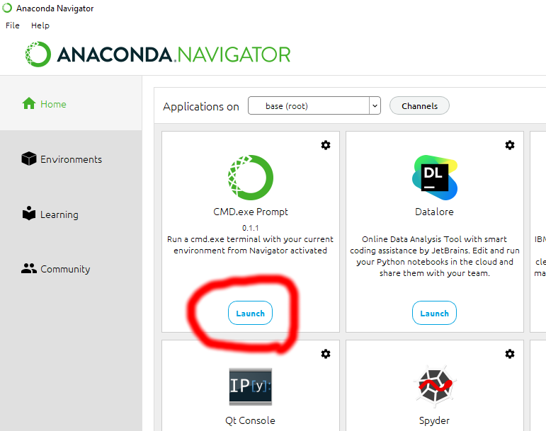
1.4.1. Windows#
In Windows, go to the Home view and click on the “Launch” button for “CMD.exe Prompt” (also known as the “Command Prompt”). The image below shows what the “Launch” button looks like:
1.4.2. Mac#
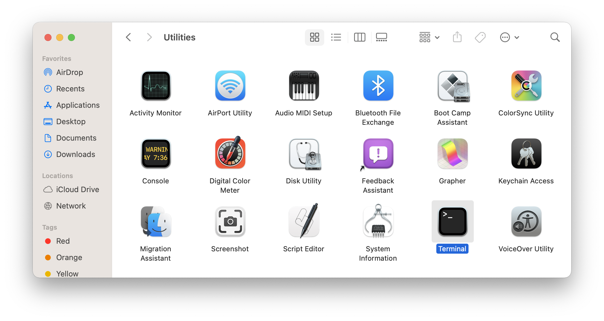
In Mac, open “Finder”, select “Applications”, click “Utilities”, and then click on the “Terminal” icon. The image below shows what the “Terminal” icon looks like:
1.4.3. Working in the shell#
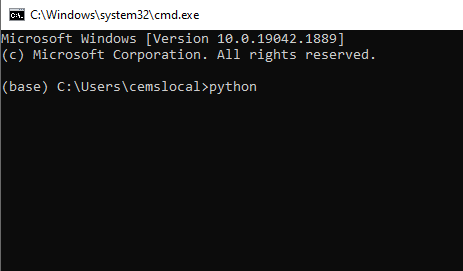
Once you have the Command Prompt (Windows) or Terminal (Mac) running, type python and press ENTER. The image below
shows this step using the Command Prompt:
Now you are in the Python interactive shell! We can start typing in commands to use Python. For example, we can use
the shell as a calculator. Let us answer the age-old question: What is one plus four? Type in 1+4 in the prompt
(after the >>>) and press ENTER on the keyboard to see the answer:
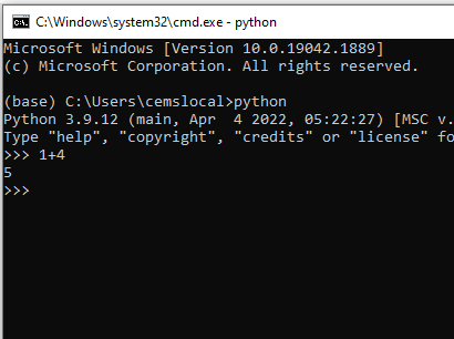
You can see we got an output right away, 5, which settles that question. This demonstrates how the interactive shell
“reads” an input using the Python interpreter, “evaluates” the result, “prints” out an output, and the “loops”
back to reading. This programming pattern is often referred to as REPL. The interactive shell is a great way to
quickly get an answer to something using Python, it simply requires typing in some commands and pressing ENTER to get a
result.
Definition: REPL
Programming pattern acronym for “read” an input, “evaluate” the result, “print” out an output, and “loop” back to read the next input.
Definition: interpreter
A program that takes in human readable code, converts it to machine code (ultimately as binary data for the computer to understand), and runs the code.
The downside of the interactive shell is that you have to retype all the commands each time you open it up. In the next section, we will explore how to store code in an external file and then have the Python interpreter parse that file.
1.5. Running Python code files#
Python code files are simply text files with a filename that ends with the file extension .py that contain Python
code. We could use simple text editors like Notepad on Windows or TextEdit on Mac to create and edit Python files.
However, programmers like to be efficient (or lazy), and want to have additional features on top of the text editor to
help them code, such as built-in error checking and automatic tab completion. Therefore, some programmers have replaced
simple text editors with “integrated development environments”, or IDEs, which have
features to help them code quickly and correctly. We will be using a Python IDE that is installed with the base
environment in Anaconda called Spyder to create and edit Python code files.
Other popular and free IDEs are PyCharm Community Edition and
VSCode.
Definition: integrated development environment (IDE)
A software application focused on creating computer code. IDEs often contain text editing, error checking, automatic formatting, and other tools to assist with efficient and correct coding.
1.5.1. Running Spyder#
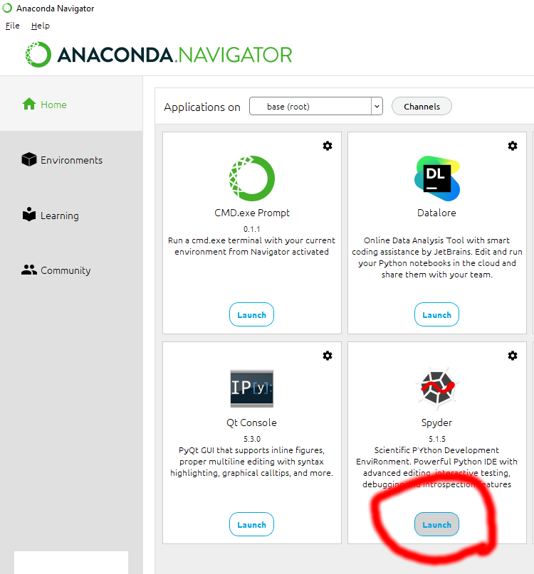
To launch Spyder, go to the Home view and click the “Launch” button below “Spyder”:
You will now see Spyder launch in its default layout:
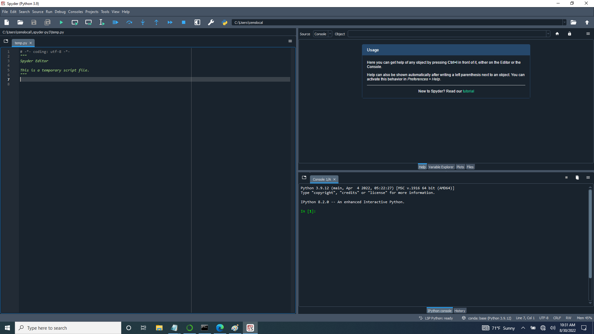
The Spyder IDE is made up of several panes that show different contextual information. You can customize what panes are visible with the “View” menu at the top of the application. We will be using the default layout.
The left side pane is the Python code editor. This is where you type Python commands to save into a file.
By default, Spyder will automatically open a temporary file called temp.py to start typing in. That will work for
now; we just have to remember to save the Python file to a different location when we need to run it.
The top right side pane contains several tabbed windows with the first one being the “Help” window that shows Python documentation and other useful information.
The bottom right side pane contains an interactive shell, just like we used before. This is handy to test out code when writing a longer Python code file.
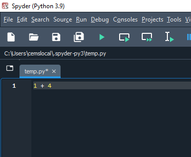
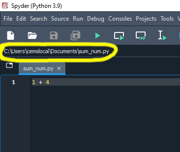
Let us try creating a Python file and running it. In the code editor pane, let us add our math equation to the Python
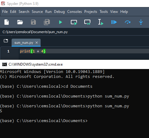
file. First, select all the contents of the file and delete it. Then type 1 + 4 for the first line:
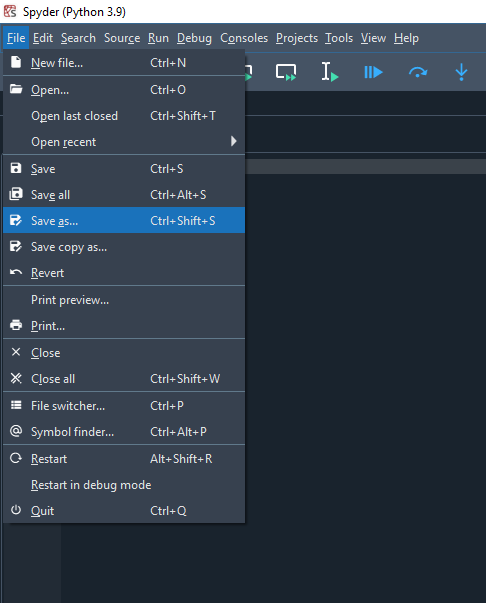
Now that we have added a line of code to our file, we need to save it. In the top menu, go to “File” and click “Save As”:
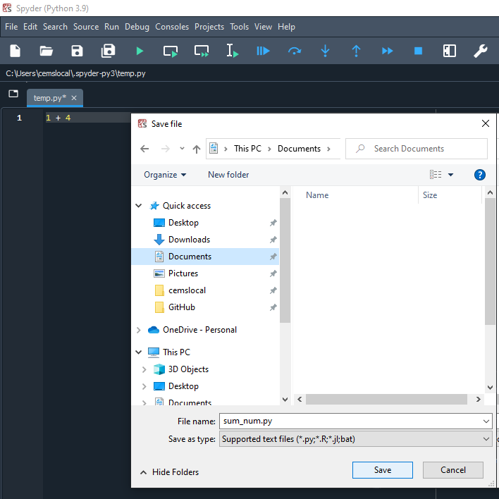
Let us save this file as “sum_num.py” in the “Documents” folder. Both Windows and Mac should have a “Documents” folder that exists in the user’s home folder. Click “Save” to save the file to the folder:
If you are ever unsure about the file path of the file you are editing, the entire file path is displayed just above the selected file, as can be seen here:
Now we can run our Python file. As we have done earlier, open up a Python interactive shell. On Windows, open the “CMD.exe Prompt” launcher in Anaconda. On Mac, open the “Terminal” app.
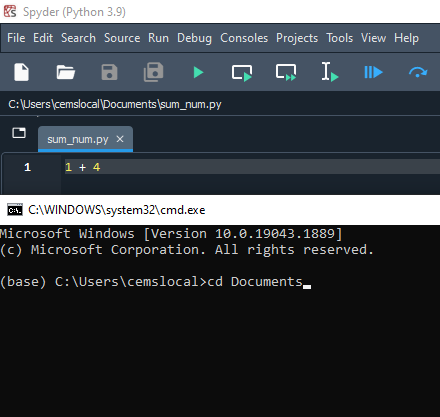
The first thing we need to do in the command prompt is move into the “Documents” folder. In the command prompt or
terminal, type cd Documents and press ENTER. The cd command stands for change directory, and we are changing into
the “Documents” folder of the home directory. Two other hints for cd:
While typing a filename, can press the TAB key to autocomplete the filename.
Type
cd ..to go back one directory level
Now that we are in the “Documents” folder, we can now run our Python file. Simply type python sum_num.py and press
ENTER. Again, you can start typing the filename, like sum_, and press the TAB key to autocomplete the filename.
Below are screenshots of running the program using the command prompt:
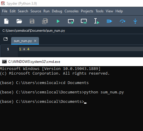
Well that is odd, we didn’t get any output! Why not? Well, when we are working in the interactive shell, the Python
interpreter follows the REPL programming pattern mentioned earlier. However, when you pass a file
directly to the Python interpreter, the shell no longer acts in an interactive mode. Instead, the Python commands in
the code file are parsed and executed exactly as written. So, to output the answer from the Python file we will need to
include the builtin print() function to our Python file, which will print out the value of the
argument that is passed to it.
Hey! Listen!
At this point, do not worry about “functions”, “arguments”, and how print() even works. We will cover all of this
in subsequent lessons.
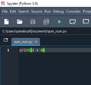
So, let us add the print() function to our code file. Delete the first line and instead type print(1 + 4).
Now “1 + 4” is being passed as an argument to the print() function, and its result will be printed out. The image
below shows print(1 + 4) being entered into our Python code file:
Now we can run our code file again and see what happens:
Perfect! Now we can write Python code files and evaluate them. This will be very useful when we write long Python programs that need to be run over and over. If you want to learn more about this useful IDE, the official documentation is a good place to start.
1.6. Running JupyterLab notebooks#
Up to this point, we have showed two different ways to execute Python code. Each way has its own advantages and disadvantages. Fortunately, the JupyterLab IDE provides an interactive computing environment that combines the interactivity of the Python shell with the long form coding format of Python files through the use of IPython notebooks (a.k.a. Jupyter notebooks). Let us open up JupyterLab to see how it works. To launch JupyterLab, go to the Home view in Anaconda Navigator and click the “Launch” button below the “JupyterLab” field:
By default, JupyterLab should open a new tab showing the JupyterLab environment in your web browser with
localhost:8888/lab in the address bar:
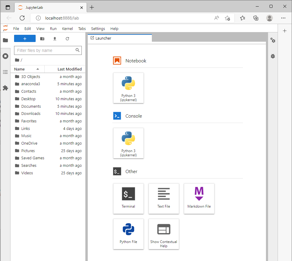
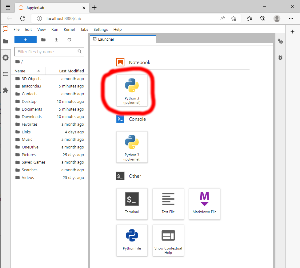
This is the JupyterLab workspace. On the left is a sidebar containing the file manager. By default, the file manager opens your user home folder as the location for browsing files. Next to the sidebar is the main editor window. This is where Python notebooks and files are displayed and edited. By default, the main editor window has a single tab open showing various JupyterLab “Launchers”. On the Launcher tab, under “Notebook”, click the “Python 3 (ipykernel)” launcher to open a new Jupyter notebook. See the red circle in the below image to the launcher:
Now we can edit our first Jupyter notebook! Below is an image of a blank IPython notebook file:
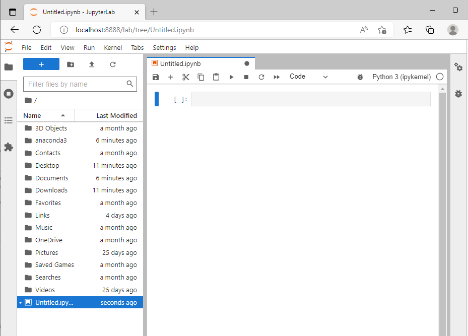
In the sidebar file manager we can see a new file is now highlighted “Untitled.ipynb”. This is our new Jupyter notebook file that we have created and are now editing. The .ipynb denotes the Jupyter lab IPython file extension, which is useful in recognizing Jupyter notebook files.
The main editor window now displays our Jupyter notebook. Select the grey rectangle in the main editor
window, which is called a code cell. Once you have selected the cell, your cursor should start blinking. Type in
1+4, press SHIFT and ENTER key at the same time (SHIFT + ENTER), and see what happens:
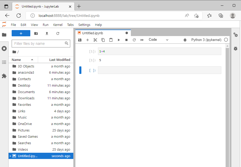
You have just run the code in that code cell! Now let us explore and explain the notebook environment some more:
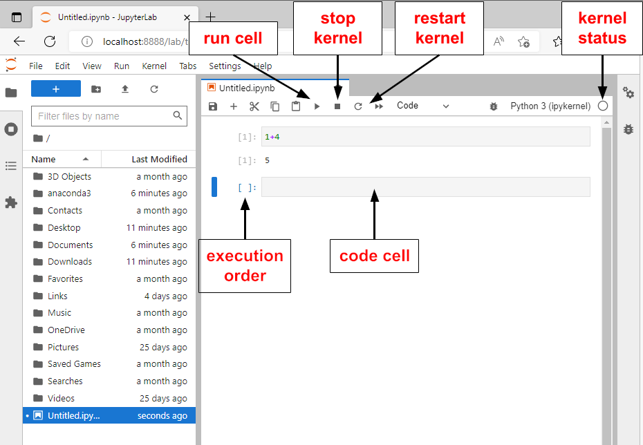
Code cell: The gray area is where you type Python code.
Execution order: The brackets next to the code cell denotes the order the cell was run. This is explained below.
Run cell: This button executes the current cell, the same action as pressing SHIFT + ENTER
Stop kernel: This button interrupts the background kernel process.
Restart kernel: This button restarts the background kernel process. This is explained further down below.
Kernel status: This circle icon denotes if the kernel is executing code or in an idle state. When empty, it is idle, when full, it is running
There are a couple of concepts that are useful to understand about the notebook environment: the kernel, the execution order of commands, and notebook management.
1.6.1. The kernel#
The kernel is a background process that executes each code cell one at a time. Like the Python interactive shell, the kernel reads the code that you’ve typed in, evaluates it, and prints out the output. The kernel starts up once you’ve opened a notebook.
The status of the kernel is displayed in the top right of the browser. When you are executing a code cell, and the kernel is processing the commands, the circle next to “Python 3 (ipykernel)” should be filled in. When execution is complete, the circle should be empty which denotes the kernel is idle.
1.6.1.1. Kernel interruption#
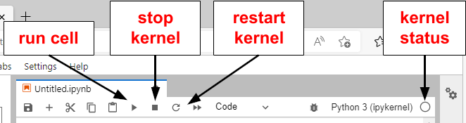
Sometimes, or more likely often, we make mistakes when coding. Perhaps we have started executing a code cell that has a mistake in it, and you’d like to stop the kernel. There are two ways to interrupt the kernel from running. One option is to click the square stop button to interrupt the kernel and halt the current execution. The image below shows the location of this button:
Alternatively, you can click the restart kernel button. This will first interrupt the kernel and then restart the entire kernel session. Clearing the kernel session means the variables that were assigned will be cleared, every code cell that has been run will be removed from memory. Code cells will have to be executed again from the beginning. Restarting the kernel is useful if you want to start your notebook again with a fresh state.
1.6.2. Execution order#
As we evaluate code cells we are changing the state of the ipython notebook. The order in which we evaluate code cells is the called the execution order. The execution order is denoted by the number in the brackets to the left of the code cell. If you were to press SHIFT + ENTER from start to end of a notebook, the kernel would evaluate all the code cells in the order they are displayed. However, you do not have to evaluate code cells in order, and in fact you can run code cells in any order you want. This is important to keep in mind to understand the output of an IPython notebook.
Here is a concrete example: How is it that print(a) outputs 16 when in the previous cell we had
just assigned a = 4 + 1?
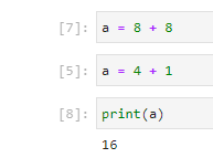
The answer is in the execution order of the cells. From the number within the brackets, the execution order,
it is clear the top cell was run ([7]), and then right away the bottom cell was run ([8]). That is why the final
output can be 16 instead of 5. At a glance this can look out of place, so it is important to note the execution
number in the brackets to follow the output in a notebook.
1.6.3. Notebook management#
Finally, a few miscellaneous notes regarding Jupyter notebook management. You can rename any Jupyter notebook by right-clicking the file name and selecting “Rename” from the context menu.
JupyterLab will autosave the Jupyter notebook every two minutes, but you can also manually save by going to the menu and clicking File -> “Save Notebook”, or using the shortcut CTRL+S on Windows or CMD+S on Mac.
1.7. Running this book as IPython notebooks#
As a reminder, you can download the entire “Introduction to Scientific Python” book as JupyterLab .ipynb notebooks.
1.8. Conclusion#
Installed Anaconda
Launched interactive shell to type commands (“CMD.exe Prompt” or “Terminal”)
Launched Spyder to edit code files
Launched JupyterLab to run notebooks