Basic Curve Fitting
Contents
1. Basic Curve Fitting#
1.1. Lesson overview#
Analyzing measured data with a theoretical model is a common task for a scientist and engineer. Often we end up “fitting” a dataset to some sort of mathematical function like a line, a sinusoid wave, or an exponentially decaying function. The fitted parameters from this analysis often end up being related to important materials properties, processing conditions, or physical phenomena.
Least squares regression is a commonly used when fitting data. You may have done this before in other software packages (e.g., Microsoft Excel’s LINEST function). In this lesson, we will go over how to do basic least squares regression analysis using the SciPy library. We first will go over how to perform a regression analysis by fitting a line through a dataset, and then we will demonstrate how perform curve fitting with a non-linear function.
1.2. Topics taught#
Performing least squares analysis using the
scipy.optimize.curve_fit()function.Reporting fitting parameters and standard errors / uncertainties.
Reading data from a file using the
numpy.loadtxt()function.Plotting measured data and fit lines with the Matplotlib library.
1.3. Line fitting#
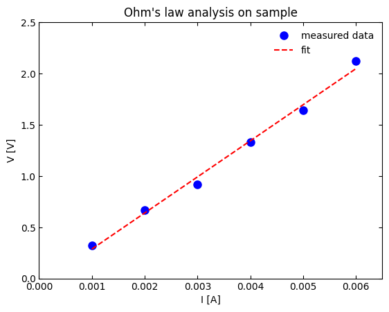
In this example, we will fit a line through a data set containing current-voltage measurements of an electronic device in order to extract the resistance of the device. As a quick review, Ohm’s law demonstrates that there is a linear relationship between the voltage across a resistor and the current passing through a resistor via the equation,
where \(V\) is the voltage across a resistor (units: volt, V), \(I\) is the current passing through a resistor (units: amps, A), and \(R\) is the inherent electrical “resistance” of the device (units: V/A = ohm). In circuit analysis, electrical devices and materials are often modeled as resistors, so measuring the resistance is a common task for a scientist or engineer.
Data for this exercise can be found in the file
IV_data_no_uncertainty.csv. This file has two columns of
data: (1) the sourced current and (2) measured voltage of the measurement. The first row has the labels for each
column and the second row has the units for each column. Since this is a CSV file, each column is separated with a ,
symbol.
We will need to use three external libraries in order to read the data file, perform the regression analysis, and plot the data and fitted line. These are the NumPy, SciPy, and Matplotlib libraries, respectively. Let’s first load the necessary libraries for the analysis:
import numpy as np
from matplotlib import pyplot as plt
from scipy.optimize import curve_fit
The import calls for the NumPy and Matplotlib libraries should be familiar to you if you have read the
Introduction to Scientific Python module (specially
the introduction to NumPy section and the
basic plotting with Matplotlib section). The
new import call in this section is for the scipy.optimize.curve_fit() function. We will review the details of this
function soon.
Now, we create the function we want to fit the data with, in this case a line. Recall that a line follows the formula,
where \(y\) is the dependent variable in the measurement (i.e., usually what is measured), \(x\) is the independent variable (i.e., usually what is sourced), \(m\) is the slope of the line, and \(b\) is the \(y\)-intercept (i.e., the \(y\) value when \(x\) = 0). The function call below creates a creates our line that will be fitted soon:
def linearFunc(x, intercept, slope):
    y = intercept + slope * x
    return y
Now let’s load our data from IV_data_no_uncertainty.csv using the numpy.loadtxt() function. We have demonstrated
how to use this function before in our
Introduction to Scientific Python module’s section on working with CSV files.
The code below loads the data to a NumPy data array called data1 and prints out the entire array to the shell just
to confirm it has been loaded correctly:
data1 = np.loadtxt("./example_data/IV_data_no_uncertainty.csv",
                   delimiter = ",",
                   skiprows = 2)
print(data1)
[[1.00e-03 3.20e-01]
 [2.00e-03 6.70e-01]
 [3.00e-03 9.20e-01]
 [4.00e-03 1.33e+00]
 [5.00e-03 1.64e+00]
 [6.00e-03 2.12e+00]]
Notice the skiprows=2 argument prevents NumPy from trying to load the header rows in the CSV file to data
array. Failure to do so would cause the following ValueError:
data_bad_import = np.loadtxt("./example_data/IV_data_no_uncertainty.csv",
                   delimiter = ",")
print(data_bad_import)
---------------------------------------------------------------------------
ValueError                                Traceback (most recent call last)
ValueError: could not convert string to float: ''

The above exception was the direct cause of the following exception:

ValueError                                Traceback (most recent call last)
Input In [4], in <cell line: 1>()
----> 1 data_bad_import = np.loadtxt("./example_data/IV_data_no_uncertainty.csv",
      2                    delimiter = ",")
      3 print(data_bad_import)

File /srv/docs_venv/lib/python3.10/site-packages/numpy/lib/npyio.py:1373, in loadtxt(fname, dtype, comments, delimiter, converters, skiprows, usecols, unpack, ndmin, encoding, max_rows, quotechar, like)
   1370 if isinstance(delimiter, bytes):
   1371     delimiter = delimiter.decode('latin1')
-> 1373 arr = _read(fname, dtype=dtype, comment=comment, delimiter=delimiter,
   1374             converters=converters, skiplines=skiprows, usecols=usecols,
   1375             unpack=unpack, ndmin=ndmin, encoding=encoding,
   1376             max_rows=max_rows, quote=quotechar)
   1378 return arr

File /srv/docs_venv/lib/python3.10/site-packages/numpy/lib/npyio.py:1016, in _read(fname, delimiter, comment, quote, imaginary_unit, usecols, skiplines, max_rows, converters, ndmin, unpack, dtype, encoding)
   1013     data = _preprocess_comments(data, comments, encoding)
   1015 if read_dtype_via_object_chunks is None:
-> 1016     arr = _load_from_filelike(
   1017         data, delimiter=delimiter, comment=comment, quote=quote,
   1018         imaginary_unit=imaginary_unit,
   1019         usecols=usecols, skiplines=skiplines, max_rows=max_rows,
   1020         converters=converters, dtype=dtype,
   1021         encoding=encoding, filelike=filelike,
   1022         byte_converters=byte_converters)
   1024 else:
   1025     # This branch reads the file into chunks of object arrays and then
   1026     # casts them to the desired actual dtype.  This ensures correct
   1027     # string-length and datetime-unit discovery (like `arr.astype()`).
   1028     # Due to chunking, certain error reports are less clear, currently.
   1029     if filelike:

ValueError: could not convert string '\ufeffI' to float64 at row 0, column 1.
Now let’s create two variables to hold the current and voltage data values:
current = data1[:, 0]
voltage = data1[:, 1]
With the data now loaded, let’s perform the least squares fit. The line of code below performs the least squares fit:
popt, pcov = curve_fit(linearFunc, current, voltage)
Notice the three positional arguments: linearFunc, current, and voltage. As detailed in the online documentation
for scipy.optimize.curve_fit(),
the first positional argument is the model function to fit with, which in our case is our linearFunc function from
earlier. The second positional argument is our independent variable data current (i.e., the “x” value in the data;
calledxdata in the
documentation).
The final positional value is our dependent variable data voltage (i.e., the “y” value in the data;
called ydata in the
documentation). There are many
additional keyword arguments that can be used, but for this basic tutorial, these will suffice.
In our call of scipy.optimize.curve_fit() we return two variables: popt and pcov. According to the
documentation, popt is a 1D
array that contains the optimized fitted parameters and pcov is a 2D array that contains the variances and
covariances of the fitted parameters. For our needs, the square root of the diagonal represents the standard errors
of the fitted parameters (a.k.a. the standard uncertainties of each parameter).
Let’s now extract the fitting parameters and their standard uncertainties with the following block of code:
intercept = popt[0]
slope = popt[1]
intercept_err = np.sqrt(pcov[0][0])
slope_err = np.sqrt(pcov[1][1])
With this block of code, we have all we need in the regression analysis! For completion, let’s make a plot that shows the optimized line with our data. The code below goes over all the necessary steps to make this happen. If you need a review on the basics of plotting, look at our Introduction to Scientific Python module’s section on basic plotting with Matplotlib.
# Create figure
fig1 = plt.figure()
ax = fig1.add_subplot(1, 1, 1)

# Plot measured data
ax.plot(current, voltage,
        label="measured data",
        marker="o",
        markersize=8,
        linestyle="none",
        color="blue")

# Create fitted line
yfit = intercept + slope * current

# Plot fit data
ax.plot(current, yfit,
        color="red",
        label="fit",
        linestyle="dashed")

# Figure options
ax.set_title("Ohm's law analysis on sample")
ax.set_xlabel("I [A]")
ax.set_ylabel("V [V]")
ax.tick_params(axis="both", direction="in")
ax.tick_params(top="on")
ax.tick_params(right="on")
ax.set_xlim(left=0, right=6.5E-3)
ax.set_ylim(bottom=0, top=2.5)
ax.legend(frameon=False)

# Show plot
plt.show()

Comments have been provided in the code above for readability. To create the fit line, we first create yfit, which
contains calculated voltages based on our input current array and the fitting results intercept and slope (notice
the line equation format). We then include this data set to the graph as an overlay.
Finally, we can also report the fitting results to the shell with a set of four print() calls. Here, we use
f-formatting of strings
and number rounding in strings
to readability purposes.
print(f"intercept = {intercept:.3f} V")
print(f"intercept std. error = {intercept_err:.3f} V")
print(f"slope = {slope:.1f} ohm")
print(f"slope std. error = {slope_err:.1f} ohm")
intercept = -0.065 V
intercept std. error = 0.058 V
slope = 352.0 ohm
slope std. error = 14.9 ohm
1.4. Non-linear curve fitting#
We can also use scipy.optimize.curve_fit() to fit datasets that do not have a linear relationship. In order to
perform “non-linear curve fitting”, we simply need to rewrite our function to our desired mathematical relationship
and account for all additional fit parameters in the code. To see this in action, first download the CSV file
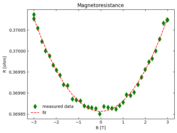
MR_data_no_uncertainty.csv, which contains a set of measured
data from a sample whose electrical resistance changes as function of magnetic field. This data will show a
second-order polynomial-like dependence (i.e., a parabola) that follows the functional form:
where \(A\) is a constant, \(B\) is the linear parameter, and \(C\) is the second-order or “quadratic” term. The block of code below is the entire code needed to fully run this regression analysis:
# Load libraries
import numpy as np
from matplotlib import pyplot as plt
from scipy.optimize import curve_fit

# Create function to fit
def parabolaFunc(x, constant, linear, quadratic):
    y = constant + linear * x + quadratic * (x**2)
    return y

# Load data and separate columns
data2 = np.loadtxt("./example_data/MR_data_no_uncertainty.csv",
                   delimiter = ",",
                   skiprows = 2)
magnetic_field = data2[:,0]
resistance = data2[:,1]

# Perform the least-squares fitting
popt, pcov = curve_fit(parabolaFunc, magnetic_field, resistance)

# Extract out the fitted parameters and standard errors
constant = popt[0]
linear = popt[1]
quadratic = popt[2]
constant_err = np.sqrt(pcov[0][0])
linear_err = np.sqrt(pcov[1][1])
quadratic_err = np.sqrt(pcov[2][2])

# Create figure
fig1 = plt.figure()
ax = fig1.add_subplot(1, 1, 1)

# Plot measured data
ax.plot(magnetic_field, resistance,
        label="measured data",
        marker="d",
        markersize=8,
        linestyle="none",
        color="green")

# Create fitted curve
yfit = constant + (linear * magnetic_field) + (quadratic * (magnetic_field**2))

# Plot fit data
ax.plot(magnetic_field, yfit,
        color="red",
        label="fit",
        linestyle="dashed")

# Figure options
ax.set_title("Magnetoresistance")
ax.set_xlabel("B [T]")
ax.set_ylabel("R [ohm]")
ax.tick_params(axis="both", direction="in")
ax.tick_params(top="on")
ax.tick_params(right="on")
#ax.set_xlim(left=0, right=2.5)
#ax.set_ylim(bottom=0.3525, top=0.3535)
ax.legend(frameon=False)

# Show plot
plt.show()

# Report values to shell
print(f"constant = {constant:.7f} ohm")
print(f"constant std. error = {constant_err:.7f} ohm")
print(f"linear = {linear:.2E} ohm/T")
print(f"linear std. error = {linear_err:.2E} ohm/T")
print(f"quadratic = {quadratic:.4E} ohm/T^2")
print(f"quadratic std. error = {quadratic_err:.2E} ohm/T^2")

constant = 0.3698562 ohm
constant std. error = 0.0000014 ohm
linear = -1.19E-08 ohm/T
linear std. error = 5.02E-07 ohm/T
quadratic = 2.4583E-05 ohm/T^2
quadratic std. error = 3.04E-07 ohm/T^2
We have reloaded the three external libraries completeness in case you would like to re-use this code block for your own
needs. Structurally, there is no real difference from the previous line fitting example. The only differences in the
code are replacing our linear function linearFunc() with the polynomial function parabolaFunc(), renaming the
variables for the measured data, and adjusting the code to handle the new fitting parameters. In short, once you know
how to perform the line fit, you can fit any other function!
1.5. Conclusion#
Hopefully you find this lesson useful in learning the basics of curve fitting. The scipy.optimize.curve_fit()
function has additional optional arguments available that go beyond the scope of this lesson.
For example, we can use the keyword argument sigma to account for any uncertainty on the y-value for each
data point in the regression analysis. This way if our data has “error bars” on the y-value for each data point,
we can include this in the fitting process. We will cover this in an upcoming lesson. There are
also ways to enter initial values for each fitting parameter and specify bounds for each value. If you are
interested in this additional options, please look at the
documentation for curve_fit().
1.6. Want to learn more?#
Wikipedia - Least Squares
Shane Burns - Data Fitting
SciPy Library - The curve_fit() Function
NumPy - Documentation Page
Matplotlib - Home Page
